40 excel charts axis labels
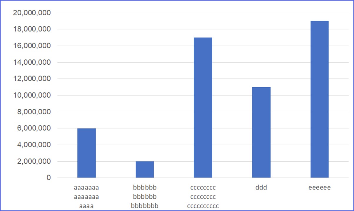
Two-Level Axis Labels (Microsoft Excel) - tips Excel automatically recognizes that you have two rows being used for the X-axis labels, and formats the chart correctly. (See Figure 1.) Since the X-axis labels appear beneath the chart data, the order of the label rows is reversed—exactly as mentioned at the first of this tip. Figure 1. Two-level axis labels are created automatically by Excel. Unable to Format Pivot Chart Axis Labels | MrExcel Message Board The axis I'm working on displays dates. The current format is MM/DD/YYYY. This is not ideal, since the chart is used to display a full month at a time. Since the text of these labels is so long, I end up with that awful "tilt your head sideways to read the labels" situation after a few weeks worth of data has been entered each month:
Excel Chart Axis Label Tricks • My Online Training Hub Chart Axis Alignment. We could use the alignment tools. Right-click axis > Format Axis > Alignment. But before you waste time doing this there is a better way. Actually there are a few options. First, you don't want your audience having to turn their head to the side to read labels. If you're plotting dates then you can:

Excel charts axis labels
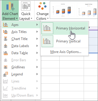
How to Label Axes in Excel: 6 Steps (with Pictures) - wikiHow Open your Excel document. Double-click an Excel document that contains a graph. If you haven't yet created the document, open Excel and click Blank workbook, then create your graph before continuing. 2 Select the graph. Click your graph to select it. 3 Click +. It's to the right of the top-right corner of the graph. This will open a drop-down menu. How to Change Axis Labels in Excel (3 Easy Methods) For changing the label of the Horizontal axis, follow the steps below: Firstly, right-click the category label and click Select Data > Click Edit from the Horizontal (Category) Axis Labels icon. Then, assign a new Axis label range and click OK. Now, press OK on the dialogue box. Finally, you will get your axis label changed. How To Add Axis Labels In Excel - BSUPERIOR 21 Jul 2020 — Method 1- Add Axis Title by The Add Chart Element Option · Click on the chart area. · Go to the Design tab from the ribbon. · Click on the Add ...
Excel charts axis labels. How to Add Axis Labels to a Chart in Excel | CustomGuide Add Data Labels · Select the chart. · Click the Chart Elements button. · Click the Data Labels check box. Gridlines, Labels, and Data Tables. In the Chart Elements ... Change the display of chart axes - support.microsoft.com On the Format tab, in the Current Selection group, click the arrow in the Chart Elements box, and then click the horizontal (category) axis. On the Design tab, in the Data group, click Select Data. In the Select Data Source dialog box, under Horizontal (Categories) Axis Labels, click Edit. In the Axis label range box, do one of the following: Edit titles or data labels in a chart - support.microsoft.com On a chart, click the chart or axis title that you want to link to a corresponding worksheet cell. On the worksheet, click in the formula bar, and then type an equal sign (=). Select the worksheet cell that contains the data or text that you want to display in your chart. You can also type the reference to the worksheet cell in the formula bar. How to rotate axis labels in chart in Excel? - ExtendOffice If you are using Microsoft Excel 2013, you can rotate the axis labels with following steps: 1. Go to the chart and right click its axis labels you will rotate, and select the Format Axis from the context menu. 2.
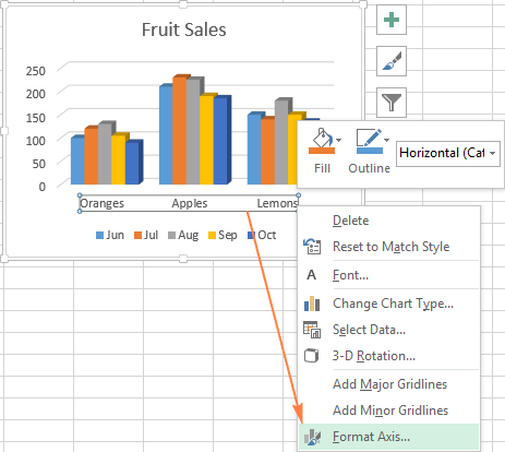
Axis Labels overlapping Excel charts and graphs • AuditExcel.co.za Stop Labels overlapping chart. There is a really quick fix for this. As shown below: Right click on the Axis. Choose the Format Axis option. Open the Labels dropdown. For label position change it to 'Low'. The end result is you eliminate the labels overlapping the chart and it is easier to understand what you are seeing . Excel Chart not showing SOME X-axis labels - Super User In Excel 2013, select the bar graph or line chart whose axis you're trying to fix. Right click on the chart, select "Format Chart Area..." from the pop up menu. A sidebar will appear on the right side of the screen. On the sidebar, click on "CHART OPTIONS" and select "Horizontal (Category) Axis" from the drop down menu. Excel Chart, Axis Label decimal removal - Super User 1) Select the axis, right-click and choose "Format Axis" from teh pop-up menu. Under "number", Enter 0 (or the number of decimal places you want) You can also choose to have negatives diaplayed in red there. Share. Improve this answer. How to group (two-level) axis labels in a chart in Excel? - ExtendOffice (1) In Excel 2007 and 2010, clicking the PivotTable > PivotChart in the Tables group on the Insert Tab; (2) In Excel 2013, clicking the Pivot Chart > Pivot Chart in the Charts group on the Insert tab. 2. In the opening dialog box, check the Existing worksheet option, and then select a cell in current worksheet, and click the OK button. 3.
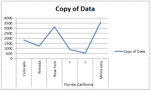
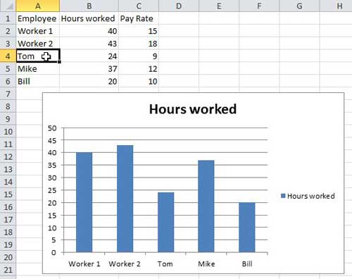
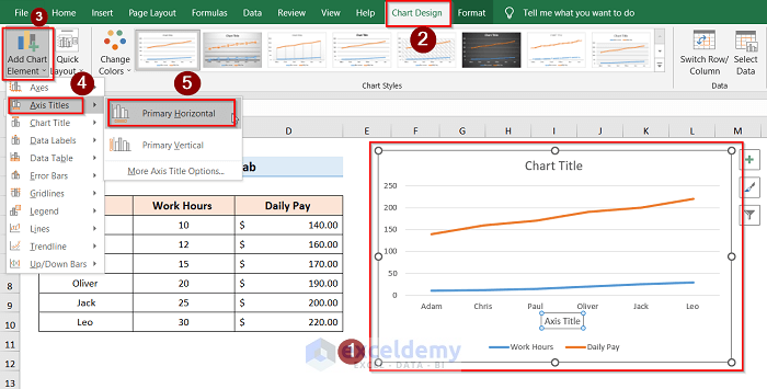
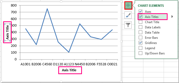
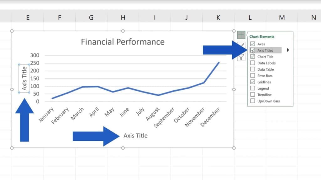
How to Add Axis Labels in Excel Charts - Step-by-Step (2022) How to add axis titles 1. Left-click the Excel chart. 2. Click the plus button in the upper right corner of the chart. 3. Click Axis Titles to put a checkmark in the axis title checkbox. This will display axis titles. 4. Click the added axis title text box to write your axis label. Change axis labels in a chart in Office - support.microsoft.com In charts, axis labels are shown below the horizontal (also known as category) axis, next to the vertical (also known as value) axis, and, in a 3-D chart, next to the depth axis. The chart uses text from your source data for axis labels. To change the label, you can change the text in the source data. How to add axis label to chart in Excel? - ExtendOffice You can insert the horizontal axis label by clicking Primary Horizontal Axis Title under the Axis Title drop down, then click Title Below Axis, and a text box will appear at the bottom of the chart, then you can edit and input your title as following screenshots shown. 4. How to display text labels in the X-axis of scatter chart in Excel? Display text labels in X-axis of scatter chart. Actually, there is no way that can display text labels in the X-axis of scatter chart in Excel, but we can create a line chart and make it look like a scatter chart. 1. Select the data you use, and click Insert > Insert Line & Area Chart > Line with Markers to select a line chart. See screenshot: 2.
Add or remove a secondary axis in a chart in Excel
How to Insert Axis Labels In An Excel Chart | Excelchat We will go to Chart Design and select Add Chart Element Figure 6 - Insert axis labels in Excel In the drop-down menu, we will click on Axis Titles, and subsequently, select Primary vertical Figure 7 - Edit vertical axis labels in Excel Now, we can enter the name we want for the primary vertical axis label.
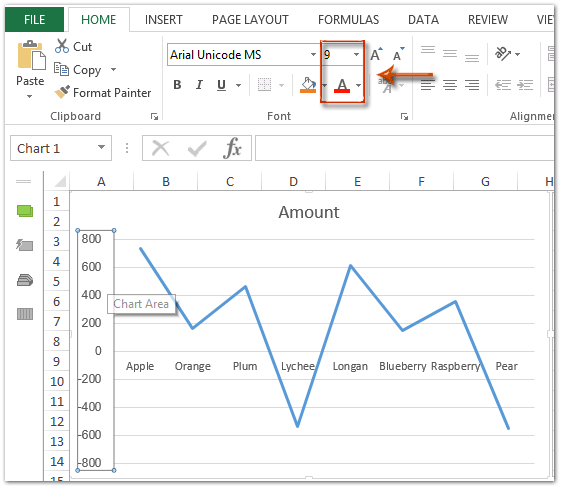
How to change chart axis labels' font color and size in Excel?
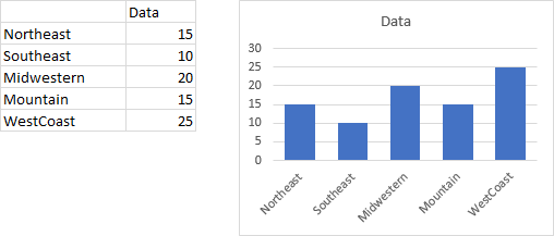
How to change Axis labels in Excel Chart - A Complete Guide In the area under the Horizontal (Category) Axis Labels box, click the Edit command button. Enter the labels you want to use in the Axis label range box, separated by commas. In the Axis label range box, enter arbitrary labels separated by commas. Click OK to confirm the chart axis labels change. Method-3: Using another Data Source
Excel axis labels - supercategory — storytelling with data
Chart Axis - Use Text Instead of Numbers - Automate Excel Change Labels. While clicking the new series, select the + Sign in the top right of the graph. Select Data Labels. Click on Arrow and click Left. 4. Double click on each Y Axis line type = in the formula bar and select the cell to reference. 5. Click on the Series and Change the Fill and outline to No Fill. 6.
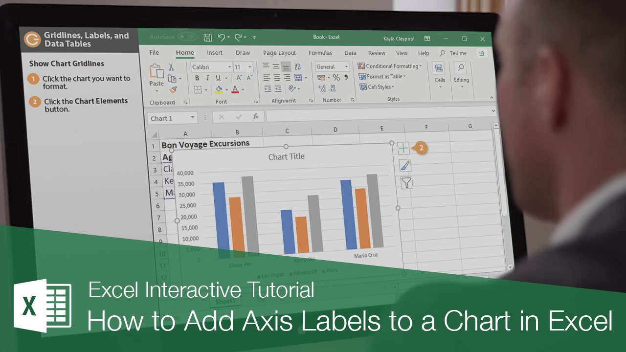
How to Add Axis Labels to a Chart in Excel | CustomGuide
Add or remove data labels in a chart - support.microsoft.com In the upper right corner, next to the chart, click Add Chart Element > Data Labels. To change the location, click the arrow, and choose an option. If you want to show your data label inside a text bubble shape, click Data Callout. To make data labels easier to read, you can move them inside the data points or even outside of the chart.

How to Change Axis Values in Excel | Excelchat
Chart.Axes method (Excel) | Microsoft Learn This example adds an axis label to the category axis on Chart1. VB With Charts ("Chart1").Axes (xlCategory) .HasTitle = True .AxisTitle.Text = "July Sales" End With This example turns off major gridlines for the category axis on Chart1. VB Charts ("Chart1").Axes (xlCategory).HasMajorGridlines = False
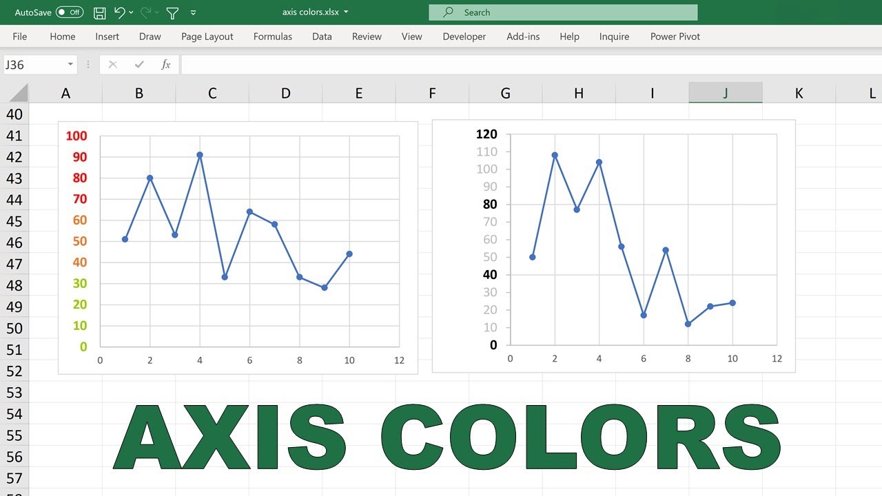
How to make the font of the axis labels different colors in an excel chart
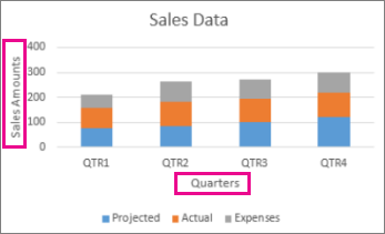
Change axis labels in a chart - support.microsoft.com Right-click the category labels you want to change, and click Select Data. In the Horizontal (Category) Axis Labels box, click Edit. In the Axis label range box, enter the labels you want to use, separated by commas. For example, type Quarter 1,Quarter 2,Quarter 3,Quarter 4. Change the format of text and numbers in labels

Bar charts with long category labels; Issue #428 November 27 ...
How to Use Cell Values for Excel Chart Labels - How-To Geek Select the chart, choose the "Chart Elements" option, click the "Data Labels" arrow, and then "More Options." Uncheck the "Value" box and check the "Value From Cells" box. Select cells C2:C6 to use for the data label range and then click the "OK" button. The values from these cells are now used for the chart data labels.
How to Wrap X Axis Labels in an Excel Chart - ExcelNotes
How to format axis labels individually in Excel - SpreadsheetWeb Double-click on the axis you want to format. Double-clicking opens the right panel where you can format your axis. Open the Axis Options section if it isn't active. You can find the number formatting selection under Number section. Select Custom item in the Category list. Type your code into the Format Code box and click Add button.

How to Add Axis Labels in Excel Charts - Step-by-Step (2022)
How to add Axis Labels (X & Y) in Excel & Google Sheets Adding Axis Labels. To add labels: Click on the Graph; Click the + Sign; Check Axis Titles. Add Axis Title Label Graph Excel.

How to Add Axis Labels to a Chart in Excel | CustomGuide
Excel Chart: Ignore Blank Axis Labels (with Easy Steps) - ExcelDemy Steps to Ignore Blank Axis Labels in Excel Chart I'm going to use the following Projects Tracking Record to show you ignore the blank axis labels in the Excel chart. The following dataset has two columns; one comprising the month names and the other has the corresponding number of projects completed. Step-1: Creating First Helper Column (HC1)

Change Horizontal Axis Values in Excel 2016 - AbsentData
Resizing Excel Charts along with axis labels, plot symbols etc. You can select and format individual chart elements just as you could in Excel. This might be what you need, but unfortunately if you resize the chart, none of the font elements resize (again, just like in Excel). When you do a Paste Special > Bitmap or any of the Picture options, you get a picture of the chart as it looked when you copied it.
Change the display of chart axes
Format Chart Axis in Excel - Axis Options Formatting a Chart Axis in Excel includes many options like Maximum / Minimum Bounds, Major / Minor units, Display units, Tick Marks, Labels, Numerical Format of the axis values, Axis value/text direction, and more. However, there are a lot more formatting options for the chart axis, in this blog, we will be working with the axis options and ...

How to Label Axes in Excel: 6 Steps (with Pictures) - wikiHow
How to change chart axis labels' font color and size in Excel? Right click the axis you will change labels when they are greater or less than a given value, and select the Format Axis from right-clicking menu. 2. Do one of below processes based on your Microsoft Excel version:

Axis Labels overlapping Excel charts and graphs • AuditExcel ...
Show Labels Instead of Numbers on the X-axis in Excel Chart We first need to create a new X and Y axis, that will be added to the existing chart. The X-axis will have the numbers from 1 to 5 and Y will have five zeroes. We will first add our X-axis by selecting the range J2:J6, then clicking on CTRL + C to copy it, then click on our chart and click CTRL+P to paste our selection.
Excel Chart Horizontal Axis Label Highlight Not Enlarged ...
Chart Axes in Excel (Easy Tutorial) To add a vertical axis title, execute the following steps. 1. Select the chart. 2. Click the + button on the right side of the chart, click the arrow next to Axis Titles and then click the check box next to Primary Vertical. 3. Enter a vertical axis title. For example, Visitors. Result: Axis Scale
How to Change Horizontal Axis Labels in Excel 2010 - Solve ...
How To Add Axis Labels In Excel - BSUPERIOR 21 Jul 2020 — Method 1- Add Axis Title by The Add Chart Element Option · Click on the chart area. · Go to the Design tab from the ribbon. · Click on the Add ...

How to Add Axis Titles in a Microsoft Excel Chart
How to Change Axis Labels in Excel (3 Easy Methods) For changing the label of the Horizontal axis, follow the steps below: Firstly, right-click the category label and click Select Data > Click Edit from the Horizontal (Category) Axis Labels icon. Then, assign a new Axis label range and click OK. Now, press OK on the dialogue box. Finally, you will get your axis label changed.

Moving the axis labels when a PowerPoint chart/graph has both ...
How to Label Axes in Excel: 6 Steps (with Pictures) - wikiHow Open your Excel document. Double-click an Excel document that contains a graph. If you haven't yet created the document, open Excel and click Blank workbook, then create your graph before continuing. 2 Select the graph. Click your graph to select it. 3 Click +. It's to the right of the top-right corner of the graph. This will open a drop-down menu.
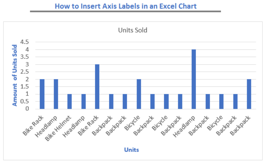
How to Insert Axis Labels In An Excel Chart | Excelchat

Two level axis in Excel chart not showing • AuditExcel.co.za

How-to Highlight Specific Horizontal Axis Labels in Excel ...

How to format axis labels individually in Excel
How to Add X and Y Axis Labels in Excel (2 Easy Methods ...

Where to Position the Y-Axis Label - PolicyViz

How to Add Axis Labels in Excel Charts - Step-by-Step (2022)

264. How can I make an Excel chart refer to column or row ...
Create a chart from start to finish
Stagger Axis Labels to Prevent Overlapping - Peltier Tech
Stagger long axis labels and make one label stand out in an ...
How to Rotate X Axis Labels in Chart - ExcelNotes
Horizontal Axis Label Highlight in an Excel Line Chart ...
Custom Axis Labels and Gridlines in an Excel Chart - Peltier Tech

Change axis labels in a chart

Change axis labels in a chart
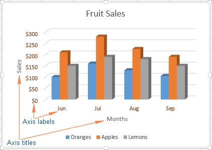
Excel charts: add title, customize chart axis, legend and ...
How to add axis label to chart in Excel?
Excel charts: add title, customize chart axis, legend and ...
How to Add Axis Titles in Excel

Stagger long axis labels and make one label stand out in an ...

How to format axis labels individually in Excel
Post a Comment for "40 excel charts axis labels"