41 multiple data labels excel pie chart

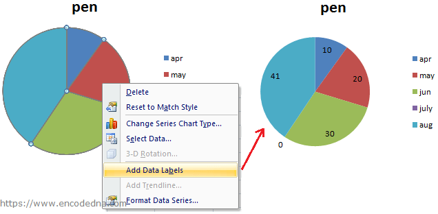
Add or remove data labels in a chart - Microsoft Support Click the data series or chart. To label one data point, after clicking the series, click that data point. In the upper right corner, next to the chart, click Add Chart Element > Data Labels. To change the location, click the arrow, and choose an option. If you want to show your data label inside a text bubble shape, click Data Callout. How to add data labels from different column in an Excel chart? This method will introduce a solution to add all data labels from a different column in an Excel chart at the same time. Please do as follows: 1. Right click the data series in the chart, and select Add Data Labels > Add Data Labels from the context menu to add data labels. 2.

Adding second set of data labels - Excel Help Forum Re: Adding second set of data labels. The chart links to workbooks on your hard drive, not to the data in the sheet. The secondary axis can only be shown when there is a series plotting on the secondary axis. Both your series are plotted on the first axis. You need to select the COUNT OF PARTS series, format it and send it to the secondary axis.

Multiple data labels excel pie chart

Change the format of data labels in a chart - Microsoft Support Tip: Make sure that only one data label is selected, and then to quickly apply custom data label formatting to the other data points in the series, click Label ... Move data labels - support.microsoft.com Click any data label once to select all of them, or double-click a specific data label you want to move. Right-click the selection > Chart Elements > Data Labels arrow, and select the placement option you want. Different options are available for different chart types. For example, you can place data labels outside of the data points in a pie ... How to Make Pie Chart with Labels both Inside and Outside 1. Right click on the pie chart, click "Add Data Labels"; · 2. Right click on the data label, click "Format Data Labels" in the dialog box; · 3.

Multiple data labels excel pie chart. How to create a pie chart in Microsoft Excel - BlogInfo You can choose to place the title above the chart or in the center. Data Labels. To change a label, select the arrow next to Data Labels in the menu. Then, you can choose from 5 different positions on the chart to display the label. ... Users can also choose from multiple color palettes for their pie charts. ... Placing an Excel pie chart into ... Quickly create multiple progress pie charts in one graph 1. Click Kutools > Charts > Difference Comparison > Progress Pie Chart to go to the Progress Pie Chart dialog box. 2. In the popped out dialog box, select the data range of the axis labels, actual values and target values under the Axis Labels, Actual Value and Target Value boxes separately. See screenshot: 3. How to Create Multi-Category Charts in Excel? - GeeksforGeeks Step 1: Insert the data into the cells in Excel. Now select all the data by dragging and then go to "Insert" and select "Insert Column or Bar Chart". A pop-down menu having 2-D and 3-D bars will occur and select "vertical bar" from it. Select the cell -> Insert -> Chart Groups -> 2-D Column Bar Chart Insertion Multi-Category Chart Excel Pie Chart Multiple Labels | Daily Catalog Add or remove data labels in a chart. Preview. 6 hours ago On the Design tab, in the Chart Layouts group, click Add Chart Element, choose Data Labels, and then click None.Click a data label one time to select all data labels in a data series or two times to select just one data label that you want to delete, and then press DELETE. Right-click a data label, and then click Delete.

Plot Multiple Data Sets on the Same Chart in Excel Follow the below steps to implement the same: Step 1: Insert the data in the cells. After insertion, select the rows and columns by dragging the cursor. Step 2: Now click on Insert Tab from the top of the Excel window and then select Insert Line or Area Chart. From the pop-down menu select the first "2-D Line". Pie Chart in Excel | How to Create Pie Chart - EDUCBA Go to the Insert tab and click on a PIE. Step 2: once you click on a 2-D Pie chart, it will insert the blank chart as shown in the below image. Step 3: Right-click on the chart and choose Select Data. Step 4: once you click on Select Data, it will open the below box. Step 5: Now click on the Add button. Create a Pie Chart in Excel (In Easy Steps) - Excel Easy Create the pie chart (repeat steps 2-3). 7. Click the legend at the bottom and press Delete. 8. Select the pie chart. 9. Click the + button on the right side of the chart and click the check box next to Data Labels. 10. Click the paintbrush icon on the right side of the chart and change the color scheme of the pie chart. Create a multi-level category chart in Excel - ExtendOffice Create a multi-level category chart in Excel A multi-level category chart can display both the main category and subcategory labels at the same time. When you have values for items that belong to different categories and want to distinguish the values between categories visually, this chart can do you a favor.

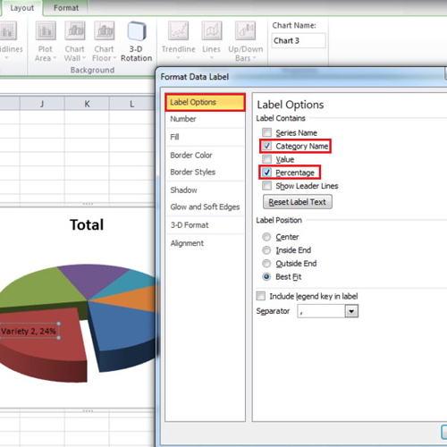
Change the format of data labels in a chart To get there, after adding your data labels, select the data label to format, and then click Chart Elements > Data Labels > More Options. To go to the appropriate area, click one of the four icons ( Fill & Line, Effects, Size & Properties ( Layout & Properties in Outlook or Word), or Label Options) shown here. How to Combine or Group Pie Charts in Microsoft Excel Click on the first chart and then hold the Ctrl key as you click on each of the other charts to select them all. Click Format > Group > Group. All pie charts are now combined as one figure. They will move and resize as one image. Choose Different Charts to View your Data Add data labels and callouts to charts in Excel 365 | EasyTweaks.com Step #1: After generating the chart in Excel, right-click anywhere within the chart and select Add labels . Note that you can also select the very handy option of Adding data Callouts. Step #2: When you select the "Add Labels" option, all the different portions of the chart will automatically take on the corresponding values in the table ... How to display leader lines in pie chart in Excel? - ExtendOffice To display leader lines in pie chart, you just need to check an option then drag the labels out. 1. Click at the chart, and right click to select Format Data Labels from context menu. 2. In the popping Format Data Labels dialog/pane, check Show Leader Lines in the Label Options section. See screenshot:

34 What Is A Data Label - Labels Design Ideas 2020

Multiple Data Labels on a Pie Chart - MrExcel Message Board #1 Hello All, So I have a table with 8 rows and 3 columns. This table includes: Column 1 - shipment name Column 2 - shipment cost Column 3 - shipment weight I have created a pie chart from this table, which covers the first two columns. Displayed next to each slice is a label with the shipment name, shipment cost, and percent share of the pie.

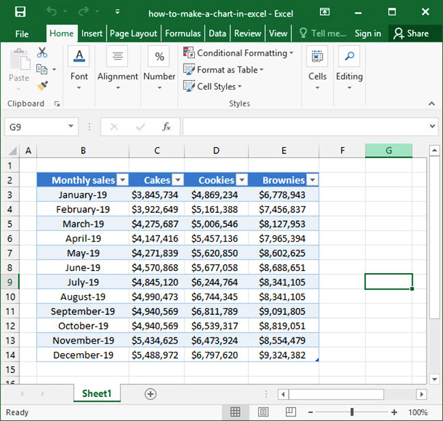
How to Create a Pie Chart in Excel using Worksheet Data

Create two data labels in pie chart? | MrExcel Message Board 30 Aug 2018 — There are 50 pie charts and I don't want to manually adjust each one. Suggestions? Excel Facts.

| Pryor Learning Solutions

How to Make a Pie Chart with Multiple Data in Excel (2 Ways) Formatting Data Labels — First, select the data set and go to the Insert tab from the ribbon. After that, click on the Pivot Chart from the Charts group.

How to Make Pie Charts and Graphs in Excel - BSUPERIOR

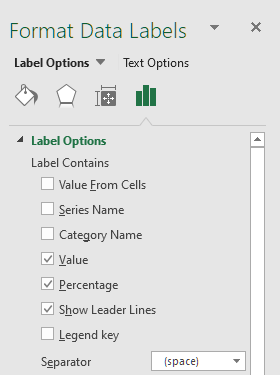
How to Make a Pie Chart in Excel (Only Guide You Need) To do this select the More Options from Data labels under the Chart Elements or by selecting the chart right click on to the mouse button and select Format Data Labels. This will open up the Format Data Label option on the right side of your worksheet. Click on the percentage. If you want the value with the percentage click on both and close it.

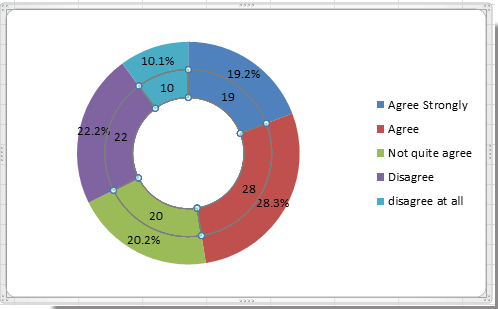
How to create doughnut chart in Excel?

Multiple Data Labels on bar chart? - Excel Help Forum Re: Multiple Data Labels on bar chart? You can mix the value and percents by creating 2 series. for the second series move it to the secondary axis and then use the %values as category labels. You can then display category information in the data labels. I have also fixed the min value to zero, which is the standard for bar/column charts.

Understanding Excel Chart Data Series, Data Points, and Data Labels

Select all Data Labels at once - Microsoft Community AFAIK it has never been possible to select all data labels (if there are multiple series) You might be able to use code like this. Sub DL () Dim ocht As Chart Dim ser As Series Dim opt As Point Dim s As Long Dim p As Long Set ocht = ActiveWindow.Selection.ShapeRange (1).Chart For s = 1 To ocht.SeriesCollection.Count

How To Make a Chart In Excel | Deskbright

Thread: Multiple data labels (in separate locations on chart) Re: Multiple data labels (in separate locations on chart) You can do it in a single chart. Create the chart so it has 2 columns of data. At first only the 1 column of data will be displayed. Move that series to the secondary axis. You can now apply different data labels to each series. Attached Files 819208.xlsx‎ (13.8 KB, 265 views) Download

How to Create and modify a pie chart in Excel | HowTech

Creating Pie Chart and Adding/Formatting Data Labels (Excel)

How to Setup a Pie Chart with no Overlapping Labels | Telerik Reporting

How to Create and Format a Pie Chart in Excel - Lifewire Select the plot area of the pie chart. Right-click the chart. Select Add Data Labels . Select Add Data Labels. In this example, the sales for each cookie is added to the slices of the pie chart. Change Colors When a chart is created in Excel, or whenever an existing chart is selected, two additional tabs are added to the ribbon.

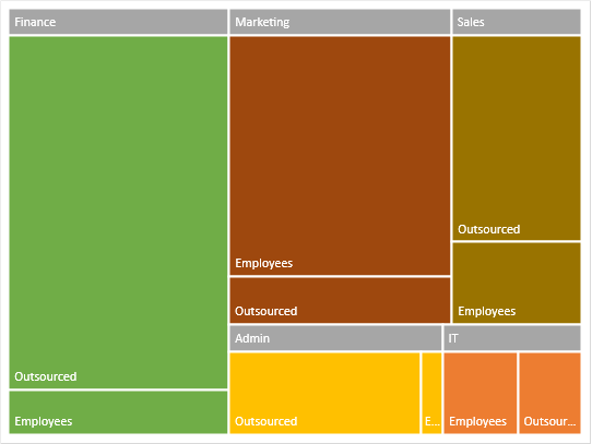
New, better alternative to Pie Charts: Treemap - Efficiency 365

Solved: Show multiple data lables on a chart - Power BI For example, I'd like to include both the total and the percent on pie chart. Or instead of having a separate legend include the series name along with the % in a pie chart. I know they can be viewed as tool tips, but this is not sufficient for my needs. Many of my charts are copied to presentations and this added data is necessary for the end ...

How to Make Better Pie Charts with On-Demand Details

Edit titles or data labels in a chart - Microsoft Support To edit the contents of a title, click the chart or axis title that you want to change. To edit the contents of a data label, click two times on the data label that you want to change. The first click selects the data labels for the whole data series, and the second click selects the individual data label. Click again to place the title or data ...

How to Make a Pie Chart in Excel & Add Rich Data Labels to The Chart!

Formatting data labels and printing pie charts on Excel for Mac 2019 ... Here's a work around I found for printing pie charts. Still can't find a solution for formatting the data labels. 1. When printing a pie chart from Excel for mac 2019, MS instructions are to select the chart only, on the worksheet > file > print. Excel is supposed to print the chart only (not the data ) and automatically fit it onto one page.

Advanced Graphs Using Excel : 3D-histogram in Excel

Everything You Need to Know About Pie Chart in Excel How to Make a Pie Chart in Excel. Start with selecting your data in Excel. If you include data labels in your selection, Excel will automatically assign them to each column and generate the chart. Go to the INSERT tab in the Ribbon and click on the Pie Chart icon to see the pie chart types. Click on the desired chart to insert.

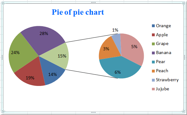
How to create pie of pie or bar of pie chart in Excel?

How to group (two-level) axis labels in a chart in Excel? Select the source data, and then click the Insert Column Chart (or Column) > Column on the Insert tab. Now the new created column chart has a two-level X axis, and in the X axis date labels are grouped by fruits. See below screen shot: Group (two-level) axis labels with Pivot Chart in Excel

Excel custom pie chart labels - Microsoft Community

How to Make Pie Chart with Labels both Inside and Outside 1. Right click on the pie chart, click "Add Data Labels"; · 2. Right click on the data label, click "Format Data Labels" in the dialog box; · 3.

Charts In Excel – Excel Tutorial World

Move data labels - support.microsoft.com Click any data label once to select all of them, or double-click a specific data label you want to move. Right-click the selection > Chart Elements > Data Labels arrow, and select the placement option you want. Different options are available for different chart types. For example, you can place data labels outside of the data points in a pie ...