42 how to show data labels in excel
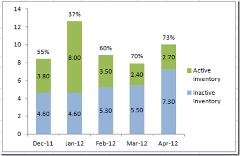
How to Add Labels to Show Totals in Stacked Column Charts in Excel In the chart, right-click the "Total" series and then, on the shortcut menu, select Add Data Labels. 9. Next, select the labels and then, in the Format Data Labels pane, under Label Options, set the Label Position to Above. 10. While the labels are still selected set their font to Bold. 11. Dynamically Label Excel Chart Series Lines - My Online Training Hub Step 1: Duplicate the Series. The first trick here is that we have 2 series for each region; one for the line and one for the label, as you can see in the table below: Select columns B:J and insert a line chart (do not include column A). To modify the axis so the Year and Month labels are nested; right-click the chart > Select Data > Edit the ...
How to create labels in Word from Excel spreadsheet May 27, 2022 · Import the Excel data into your Word document; Add the labels from Excel to Microsoft Word; Create the labels from Excel in Word; Save the document as PDF; 1] Use Microsoft Excel to enter data for ...

How to show data labels in excel
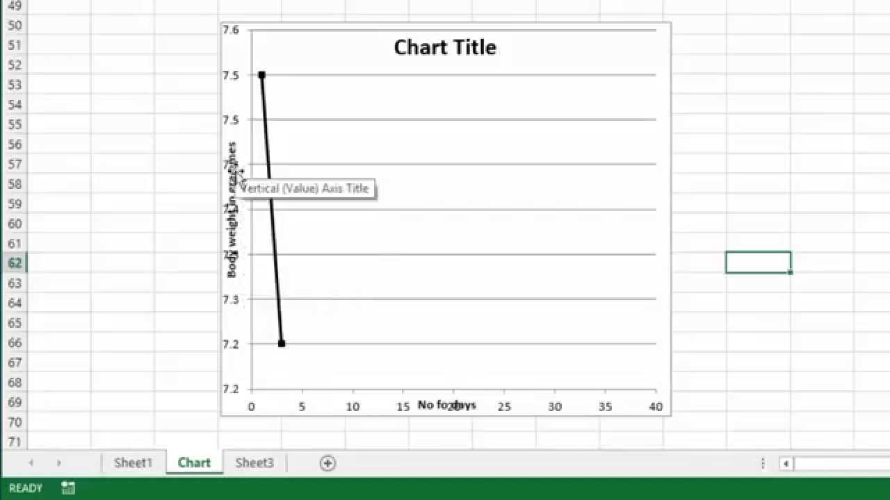
Excel charts: add title, customize chart axis, legend and data labels ... Click anywhere within your Excel chart, then click the Chart Elements button and check the Axis Titles box. If you want to display the title only for one axis, either horizontal or vertical, click the arrow next to Axis Titles and clear one of the boxes: Click the axis title box on the chart, and type the text. Add a DATA LABEL to ONE POINT on a chart in Excel Click on the chart line to add the data point to. All the data points will be highlighted. Click again on the single point that you want to add a data label to. Right-click and select ' Add data label ' This is the key step! Right-click again on the data point itself (not the label) and select ' Format data label '. How to Use Cell Values for Excel Chart Labels Mar 12, 2020 · Make your chart labels in Microsoft Excel dynamic by linking them to cell values. When the data changes, the chart labels automatically update. In this article, we explore how to make both your chart title and the chart data labels dynamic. We have the sample data below with product sales and the difference in last month’s sales.
How to show data labels in excel. How to add data labels from different column in an Excel chart? Click any data label to select all data labels, and then click the specified data label to select it only in the chart. 3. Go to the formula bar, type =, select the corresponding cell in the different column, and press the Enter key. See screenshot: 4. Repeat the above 2 - 3 steps to add data labels from the different column for other data points. › xlpivot05How to Control Excel Pivot Table with Field Setting Options Jul 10, 2021 · Check the 'Show items with no data' check box. Click OK; Show all the data in Excel 2003. Make the following change for each field in which you want to see all the data: Double-click the field button, to open the PivotTable field dialog box. Check the 'Show items with no data' check box. Click OK; Missing Data in Pivot Table How to Add Labels to Scatterplot Points in Excel - Statology Step 3: Add Labels to Points Next, click anywhere on the chart until a green plus (+) sign appears in the top right corner. Then click Data Labels, then click More Options… In the Format Data Labels window that appears on the right of the screen, uncheck the box next to Y Value and check the box next to Value From Cells. Change the format of data labels in a chart To get there, after adding your data labels, select the data label to format, and then click Chart Elements > Data Labels > More Options. To go to the appropriate area, click one of the four icons ( Fill & Line, Effects, Size & Properties ( Layout & Properties in Outlook or Word), or Label Options) shown here.
support.microsoft.com › en-us › officeMove data labels - support.microsoft.com If data labels you added to your chart are in the way of your data visualization—or you simply want to move them elsewhere—you can change their placement by picking another location or by dragging them to the location you want. Click any data label once to select all of them, or double-click a specific data label you want to move. Excel charts: how to move data labels to legend - Microsoft Tech Community You can't do that, but you can show a data table below the chart instead of data labels: Click anywhere on the chart. On the Design tab of the ribbon (under Chart Tools), in the Chart Layouts group, click Add Chart Element > Data Table > With Legend Keys (or No Legend Keys if you prefer) Add or remove data labels in a chart - support.microsoft.com Click Label Options and under Label Contains, select the Values From Cells checkbox. When the Data Label Range dialog box appears, go back to the spreadsheet and select the range for which you want the cell values to display as data labels. When you do that, the selected range will appear in the Data Label Range dialog box. Then click OK. Excel tutorial: Dynamic min and max data labels =IF (OR (C5=MAX (amounts),C5=MIN (amounts)), C5,"") The formula reads if C5 is the max of amounts, or the min of amounts, return C5. Otherwise, return an empty string. Now the formula returns both min and max values, and the chart shows these values as data labels.
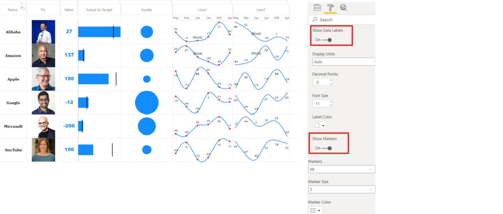
Enable or Disable Excel Data Labels at the click of a button - How To Enable/Distable Data labels using form controls - Step by Step Step 1: Here is the sample data. Select and to go Insert tab > Charts group > Click column charts button > click 2D column chart. This will insert a new chart in the worksheet. Understanding Excel Chart Data Series, Data Points, and Data Labels These are commonly used for pie charts. Percentage Labels: Calculated by dividing the individual fields in a series by the total value of the series. Percentage labels are commonly used for pie charts. Data Series: A group of related data points or markers that are plotted in charts and graphs. Examples of a data series include individual lines ... How to find, highlight and label a data point in Excel scatter plot Select the Data Labels box and choose where to position the label. By default, Excel shows one numeric value for the label, y value in our case. To display both x and y values, right-click the label, click Format Data Labels…, select the X Value and Y value boxes, and set the Separator of your choosing: Label the data point by name How to create Custom Data Labels in Excel Charts Add default data labels. Click on each unwanted label (using slow double click) and delete it. Select each item where you want the custom label one at a time. Press F2 to move focus to the Formula editing box. Type the equal to sign. Now click on the cell which contains the appropriate label. Press ENTER.

Changing Axis Labels in PowerPoint 2013 | PowerPoint Tutorials
Excel, giving data labels to only the top/bottom X% values 1) Create a data set next to your original series column with only the values you want labels for (again, this can be formula driven to only select the top / bottom n values). See column D below. 2) Add this data series to the chart and show the data labels. 3) Set the line color to No Line, so that it does not appear! 4) Volia! See Below! Share

How to set and format data labels for Excel charts in C#
How to Add Data Labels to an Excel 2010 Chart - dummies Use the following steps to add data labels to series in a chart: Click anywhere on the chart that you want to modify. On the Chart Tools Layout tab, click the Data Labels button in the Labels group. None: The default choice; it means you don't want to display data labels. Center to position the data labels in the middle of each data point.
Multiple Sparklines – Power BI & Excel are better together
Custom Chart Data Labels In Excel With Formulas Follow the steps below to create the custom data labels. Select the chart label you want to change. In the formula-bar hit = (equals), select the cell reference containing your chart label's data. In this case, the first label is in cell E2. Finally, repeat for all your chart laebls.

Microsoft Tips with Temo!: How to Add Data Labels to an Excel 2010 Chart
How to Print Address Labels From Excel? (with Examples) Enter data into column A. Press CTRL+E to start the excel macro. Enter the number of columns to print the labels. Then, the data is displayed. Set the custom margins as top=0.5, bottom=0.5, left=0.21975, and right=0.21975. Set scaling option to "Fits all columns on one page" in the print settings and click on print.

Format Data Labels in Excel- Instructions | Microsoft excel, Microsoft ...
chandoo.org › wp › change-data-labels-in-chartsHow to Change Excel Chart Data Labels to Custom Values? Now, click on any data label. This will select "all" data labels. Now click once again. At this point excel will select only one data label. Go to Formula bar, press = and point to the cell where the data label for that chart data point is defined. Repeat the process for all other data labels, one after another. See the screencast. Points to note:
Adding Data Labels To An Excel Chart | Free Microsoft Excel Tutorials
› charts › axis-labelsHow to add Axis Labels (X & Y) in Excel & Google Sheets Excel offers several different charts and graphs to show your data. In this example, we are going to show a line graph that shows revenue for a company over a five-year period. In the below example, you can see how essential labels are because in this below graph, the user would have trouble understanding the amount of revenue over this period.
Excel Dashboard Templates How-to Put Percentage Labels on Top of a ...
How to Add Data Labels in Excel - Excelchat | Excelchat In Excel 2013 and the later versions we need to do the followings; Click anywhere in the chart area to display the Chart Elements button Figure 5. Chart Elements Button Click the Chart Elements button > Select the Data Labels, then click the Arrow to choose the data labels position. Figure 6. How to Add Data Labels in Excel 2013 Figure 7.
Resize the Plot Area in Excel Chart - Titles and Labels Overlap - YouTube
Hiding data labels for some, not all values in a series Here's a good challenge for you. I can't figure it out, and I believe it's a limitation of Excel. I have a bar graph with several data series. I know how to show the data labels for every data point in a given series. But I'm looking to show the data label for only some data points in a given series -- i.e. non-zero valued data points.
Label Template Excel | printable label templates
Directly Labeling in Excel - Evergreen Data There are two ways to do this. Way #1. Click on one line and you'll see how every data point shows up. If we add a label to every data points, our readers are going to mount a recall election. So carefully click again on just the last point on the right. Now right-click on that last point and select Add Data Label.
Excel Dashboard Templates How-to Put Percentage Labels on Top of a ...
Format Data Labels in Excel- Instructions - TeachUcomp, Inc. To do this, click the "Format" tab within the "Chart Tools" contextual tab in the Ribbon. Then select the data labels to format from the "Chart Elements" drop-down in the "Current Selection" button group. Then click the "Format Selection" button that appears below the drop-down menu in the same area.

35 How To Label In Excel - Labels Database 2020
› make-labels-with-excel-4157653How to Print Labels From Excel - Lifewire Select Mailings > Write & Insert Fields > Update Labels . Once you have the Excel spreadsheet and the Word document set up, you can merge the information and print your labels. Click Finish & Merge in the Finish group on the Mailings tab. Click Edit Individual Documents to preview how your printed labels will appear. Select All > OK .

Changing Axis Labels in PowerPoint 2011 for Mac
How to wrap X axis labels in a chart in Excel? - ExtendOffice And you can wrap other labels with the same way. In our example, we replace all labels with corresponding formulas in the source data, and you can see all labels in the chart axis are wrapped in the below screen shot: Notes: (1) If the chart area is still too narrow to show all wrapped labels, the labels will keep rotated and slanted.

How to Make Charts and Graphs in Excel | Smartsheet
Excel tutorial: How to use data labels Generally, the easiest way to show data labels to use the chart elements menu. When you check the box, you'll see data labels appear in the chart. If you have more than one data series, you can select a series first, then turn on data labels for that series only. You can even select a single bar, and show just one data label.

30 What Is A Data Label In Excel - Labels Database 2020
How to add or move data labels in Excel chart? - ExtendOffice 1. Click the chart to show the Chart Elements button . 2. Then click the Chart Elements, and check Data Labels, then you can click the arrow to choose an option about the data labels in the sub menu. See screenshot:

30 How To Add Label To Excel Chart - Labels Database 2020
› charts › dynamic-chart-dataCreate Dynamic Chart Data Labels with Slicers - Excel Campus Feb 10, 2016 · Step 3: Use the TEXT Function to Format the Labels. Typically a chart will display data labels based on the underlying source data for the chart. In Excel 2013 a new feature called “Value from Cells” was introduced. This feature allows us to specify the a range that we want to use for the labels.

Creating Pie Chart and Adding/Formatting Data Labels (Excel) - YouTube
How to show data label in "percentage" instead of - Microsoft Community Select Format Data Labels Select Number in the left column Select Percentage in the popup options In the Format code field set the number of decimal places required and click Add. (Or if the table data in in percentage format then you can select Link to source.) Click OK Regards, OssieMac Report abuse 8 people found this reply helpful ·

How to Add Data Labels in Excel - Excelchat | Excelchat
How to Use Cell Values for Excel Chart Labels Mar 12, 2020 · Make your chart labels in Microsoft Excel dynamic by linking them to cell values. When the data changes, the chart labels automatically update. In this article, we explore how to make both your chart title and the chart data labels dynamic. We have the sample data below with product sales and the difference in last month’s sales.
Post a Comment for "42 how to show data labels in excel"